https://geocompr.robinlovelace.net/adv-map.html https://r-spatial.org/r/2018/10/25/ggplot2-sf.html https://cran.r-project.org/web/packages/graticule/vignettes/graticule.html
# Prepare data
# Load libraries and dependences
library(sdmpredictors)
library(ggplot2)
library(rnaturalearth)
library(raster)
library(sf)
library(stars)
# Define the extent of the map
cExtent <- c(-180,180,45,90)
# Load sea ice thickness raster data
iceMapMin <- load_layers("BO21_icethickltmin_ss")
iceMapMax <- load_layers("BO21_icethickltmax_ss")
# Load a polygon defining landmasses
worldMap <- ne_countries(scale = 10, returnclass = "sp")
# Transform sea ice thickness in a binomial surface depicting presence / absence of sea ice
iceMapMin[iceMapMin > 0] <- 1 ; iceMapMin[iceMapMin == 0] <- NA
iceMapMax[iceMapMax > 0] <- 1 ; iceMapMax[iceMapMax == 0] <- NA
# Transform sea ice data raster to polygon data
iceMapMin <- as_Spatial(st_as_sf(st_as_stars(iceMapMin), as_points = FALSE, merge = TRUE) )
iceMapMax <- as_Spatial(st_as_sf(st_as_stars(iceMapMax), as_points = FALSE, merge = TRUE) )
# Crop ice data to the final exent
iceMapMin <- crop(gBuffer(iceMapMin, byid=TRUE, width=0),cExtent)
iceMapMax <- crop(gBuffer(iceMapMax, byid=TRUE, width=0),cExtent)
# Crop landmasses to the final exent
worldMap <- crop(worldMap,cExtent)
worldMap <- aggregate(worldMap,dissolve=T)
worldMap <- gSimplify(worldMap, tol = 0.05, topologyPreserve = TRUE)
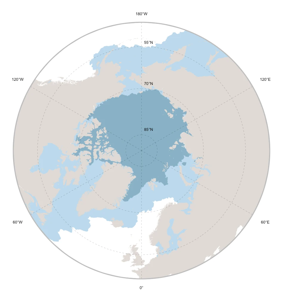
# polar map
x_lines <- seq(-120,180, by = 60)
iceMap <- ggplot() +
geom_polygon(data = iceMapMax, aes(x = long, y = lat, group = group), fill="#BCD9EC", colour = NA) +
geom_path(data = iceMapMax, aes(x = long, y = lat, group = group), color = "#BCD9EC", size = 0.1) +
geom_polygon(data = iceMapMin, aes( x = long, y = lat, group = group), fill="#89B2C7", colour = NA) +
geom_path(data = iceMapMin, aes(x = long, y = lat, group = group), color = "#89B2C7", size = 0.1) +
geom_polygon(data = worldMap, aes(x = long, y = lat, group = group), fill="#E0DAD5", colour = NA) +
theme(legend.position = "none") +
theme(text = element_text(family = "Helvetica", color = "#22211d")) +
theme(panel.background = element_blank(), axis.ticks=element_blank()) +
coord_map("ortho", orientation = c(90, 0, 0)) +
scale_y_continuous(breaks = seq(45, 90, by = 5), labels = NULL) +
scale_x_continuous(breaks = NULL) + xlab("") + ylab("") +
geom_text(size=3.5 , aes(x = 180, y = seq(53.3, 83.3, by = 15), hjust = -0.3, label = paste0(seq(55, 85, by = 15), "°N"))) +
geom_text(size=3.5 , aes(x = x_lines, y = (41 + c(-3,-3,0,-3,-3,0)), label = c("120°W", "60°W", "0°", "60°E", "120°E", "180°W"))) +
geom_hline(aes(yintercept = 45), size = 0.5, colour = "gray") +
geom_segment(size = 0.1,aes(y = 45, yend = 90, x = x_lines, xend = x_lines), linetype = "dashed") +
geom_segment(size = 1.2 ,aes(y = 45, yend = 45, x = -180, xend = 0), colour = "gray") +
geom_segment(size = 1.2 ,aes(y = 45, yend = 45, x = 180, xend = 0), colour = "gray") +
geom_segment(size = 0.1 ,aes(y = 55, yend = 55, x = -180, xend = 0), linetype = "dashed") +
geom_segment(size = 0.1 ,aes(y = 55, yend = 55, x = 180, xend = 0), linetype = "dashed") +
geom_segment(size = 0.1 ,aes(y = 70, yend = 70, x = -180, xend = 0), linetype = "dashed") +
geom_segment(size = 0.1 ,aes(y = 70, yend = 70, x = 180, xend = 0), linetype = "dashed") +
geom_segment(size = 0.1 ,aes(y = 85, yend = 85, x = -180, xend = 0), linetype = "dashed") +
geom_segment(size = 0.1 ,aes(y = 85, yend = 85, x = 180, xend = 0), linetype = "dashed")
iceMap
# Load libraries and dependences
library(sdmpredictors)
library(ggplot2)
library(rnaturalearth)
library(raster)
library(sf)
library(stars)
# Define the extent of the map
cExtent <- c(-180,180,45,90)
# Load sea ice thickness raster data
iceMapMin <- load_layers("BO21_icethickltmin_ss")
iceMapMax <- load_layers("BO21_icethickltmax_ss")
# Load a polygon defining landmasses
worldMap <- ne_countries(scale = 10, returnclass = "sp")
# Transform sea ice thickness in a binomial surface depicting presence / absence of sea ice
iceMapMin[iceMapMin > 0] <- 1 ; iceMapMin[iceMapMin == 0] <- NA
iceMapMax[iceMapMax > 0] <- 1 ; iceMapMax[iceMapMax == 0] <- NA
# Transform sea ice data raster to polygon data
iceMapMin <- as_Spatial(st_as_sf(st_as_stars(iceMapMin), as_points = FALSE, merge = TRUE) )
iceMapMax <- as_Spatial(st_as_sf(st_as_stars(iceMapMax), as_points = FALSE, merge = TRUE) )
# Crop ice data to the final exent
iceMapMin <- crop(gBuffer(iceMapMin, byid=TRUE, width=0),cExtent)
iceMapMax <- crop(gBuffer(iceMapMax, byid=TRUE, width=0),cExtent)
# Crop landmasses to the final exent
worldMap <- crop(worldMap,cExtent)
worldMap <- aggregate(worldMap,dissolve=T)
worldMap <- gSimplify(worldMap, tol = 0.05, topologyPreserve = TRUE)
# polar map
x_lines <- seq(-120,180, by = 60)
iceMap <- ggplot() +
geom_polygon(data = iceMapMax, aes(x = long, y = lat, group = group), fill="#BCD9EC", colour = NA) +
geom_path(data = iceMapMax, aes(x = long, y = lat, group = group), color = "#BCD9EC", size = 0.1) +
geom_polygon(data = iceMapMin, aes( x = long, y = lat, group = group), fill="#89B2C7", colour = NA) +
geom_path(data = iceMapMin, aes(x = long, y = lat, group = group), color = "#89B2C7", size = 0.1) +
geom_polygon(data = worldMap, aes(x = long, y = lat, group = group), fill="#E0DAD5", colour = NA) +
theme(legend.position = "none") +
theme(text = element_text(family = "Helvetica", color = "#22211d")) +
theme(panel.background = element_blank(), axis.ticks=element_blank()) +
coord_map("ortho", orientation = c(90, 0, 0)) +
scale_y_continuous(breaks = seq(45, 90, by = 5), labels = NULL) +
scale_x_continuous(breaks = NULL) + xlab("") + ylab("") +
geom_text(size=3.5 , aes(x = 180, y = seq(53.3, 83.3, by = 15), hjust = -0.3, label = paste0(seq(55, 85, by = 15), "°N"))) +
geom_text(size=3.5 , aes(x = x_lines, y = (41 + c(-3,-3,0,-3,-3,0)), label = c("120°W", "60°W", "0°", "60°E", "120°E", "180°W"))) +
geom_hline(aes(yintercept = 45), size = 0.5, colour = "gray") +
geom_segment(size = 0.1,aes(y = 45, yend = 90, x = x_lines, xend = x_lines), linetype = "dashed") +
geom_segment(size = 1.2 ,aes(y = 45, yend = 45, x = -180, xend = 0), colour = "gray") +
geom_segment(size = 1.2 ,aes(y = 45, yend = 45, x = 180, xend = 0), colour = "gray") +
geom_segment(size = 0.1 ,aes(y = 55, yend = 55, x = -180, xend = 0), linetype = "dashed") +
geom_segment(size = 0.1 ,aes(y = 55, yend = 55, x = 180, xend = 0), linetype = "dashed") +
geom_segment(size = 0.1 ,aes(y = 70, yend = 70, x = -180, xend = 0), linetype = "dashed") +
geom_segment(size = 0.1 ,aes(y = 70, yend = 70, x = 180, xend = 0), linetype = "dashed") +
geom_segment(size = 0.1 ,aes(y = 85, yend = 85, x = -180, xend = 0), linetype = "dashed") +
geom_segment(size = 0.1 ,aes(y = 85, yend = 85, x = 180, xend = 0), linetype = "dashed")
iceMap
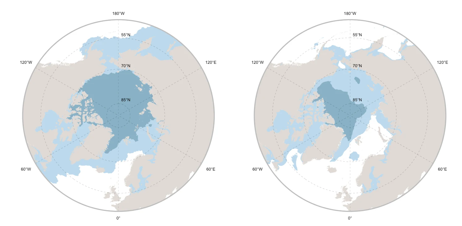
With a set of additional code lines it is possible to generate a projection of sea ice extent for the future (year 2100), here with an example under the Representative Concentration Scenario 6.0.
iceMapMin <- load_layers("BO21_RCP60_2100_icethickltmin_ss")
iceMapMax <- load_layers("BO21_RCP60_2100_icethickltmax_ss")
library(gridExtra)
grid.arrange(iceMapPresent, iceMapFuture, ncol=2)
iceMapMax <- load_layers("BO21_RCP60_2100_icethickltmax_ss")
library(gridExtra)
grid.arrange(iceMapPresent, iceMapFuture, ncol=2)