The major cause of global sea-level change is the exchange of water between ice and ocean during ice ages. The Last Glacial Maximum (LGM) was the most recent period with ice sheets at their greatest extent (maximum coverage between 26,500 and 19,000 years ago).
Massive ice sheets covered much of Northern Europe, North America and Asia and significantly affected global climate with increasing drought and desertification. Sea levels dropped about 120 meters (about 410 feet) when compared to today. This lead to exposed continental shelves, joined land masses and extensive coastal plains.
Here are a few lines of R code to produce a landmass shapefile of the Last Glacial Maximum for Geographic Information Systems. The code uses a bathymetry raster layer extracted from Bio-ORACLE, an open source dataset of GIS layers that provides geophysical, biotic and environmental data for surface and benthic marine realms.
The first section of the code reclassifies bathymetry to a binomial layer where depths above -120m are considered as landmass.
library(rgdal)
library(rgeos)
bathymetryFile <- "https://github.com/jorgeassis/rGIS/blob/master/Data/BathymetryDepthMean.tif"
bathymetry <- raster(bathymetryFile)
rclmat <- matrix(c(-Inf,-121,NA,-120,0,1,NA,NA,1), ncol=3, byrow=TRUE)
bathymetry <- reclassify(bathymetry, rclmat)
plot(bathymetry)
The second section uses a simple function to transform the binomial layer into a polygon. This is saved as a shapefile for Geographic Information Systems.
plot(bathymetryPoly)
writeOGR(bathymetryPoly, ".", "landmassLGMPolygon", driver="ESRI Shapefile")
The third section uses ggplot package to produce a map with landmass of the Last Glacial Maximum.
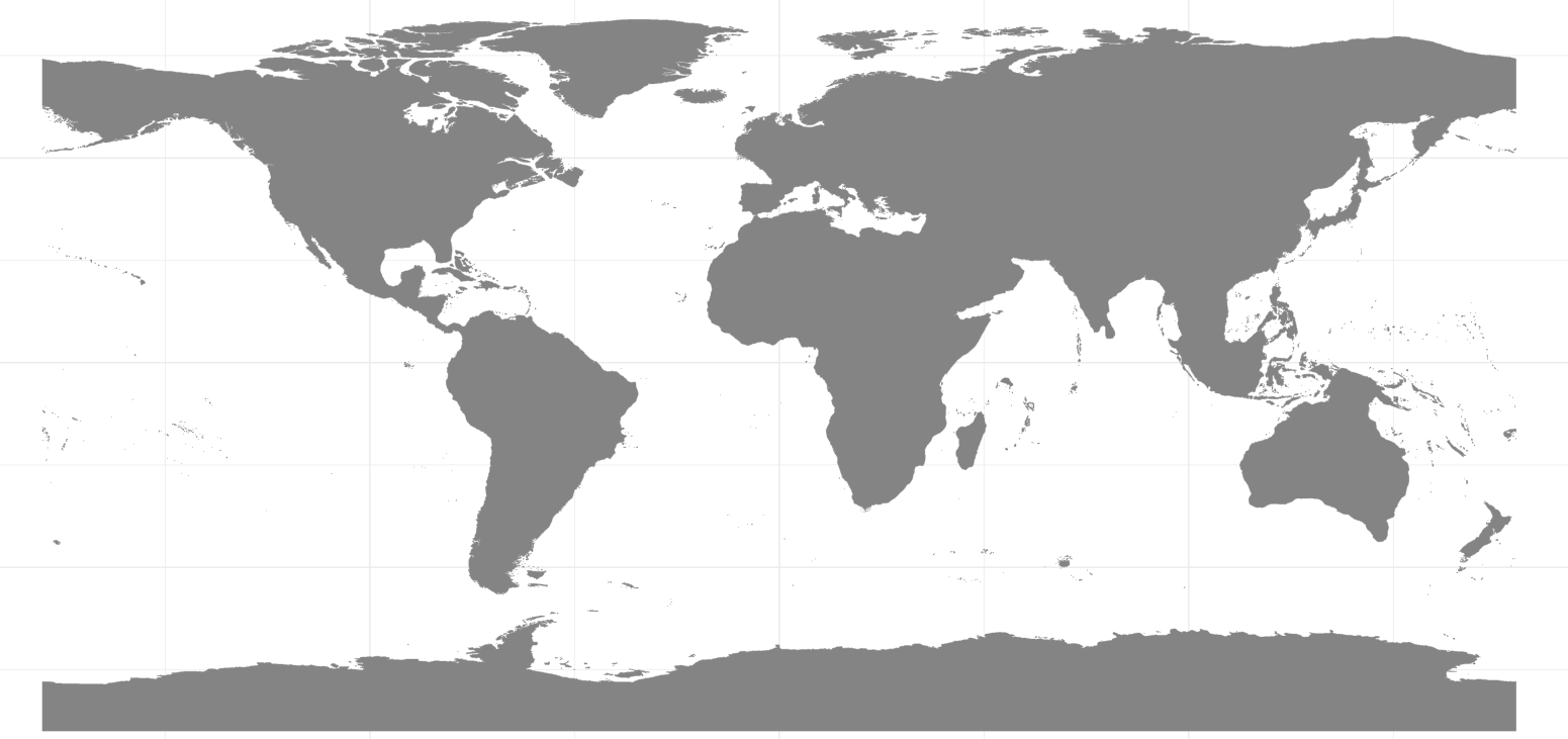
geom_polygon(data = bathymetryPoly, aes(x = long, y = lat, group = group), fill="#848484", colour = NA) +
geom_path(data = bathymetryPoly, aes(x = long, y = lat, group = group), color = "#848484", size = 0.1) +
coord_equal() +
theme_minimal() +
theme( axis.text = element_blank(),axis.ticks = element_blank(),axis.title = element_blank() )