Species distribution models (SDM; for review and definition see, e.g., Peterson et al., 2011) are a dominant paradigm to quantify the relationship between environmental dynamics and several manifestations of species biogeography. These statistical approaches pushed an emerging body of research describing the global distribution of species, addressing niche-based questions, supporting biodiversity conservation and ecosystem-based management, as well as inferring the likely anthropogenic pressures leading to population turnover and extinction.

Spatial autocorrelation (SA) is a common challenge while modelling the distribution and abundance of species. This phenomenon, likely present in most ecological datasets, denotes the situation where the values of variables sampled at nearby locations are not independent due to correlation with values at nearby locations (i.e., the value of a predictor variable at a given site can be partially predicted by the values at neighbouring sites).

Accounting for SA has not received much attention in applied SDM studies, however, when present, it may result in poorly specified models and inappropriate spatial inference and prediction. Recent studies proposed to incorporate SA into the actual models while predicting distributions (coined ‘spatial models’; Dormann, 2007), however, this approach does not allow to transfer models to new independent data (e.g., temporal and spatial transferability).

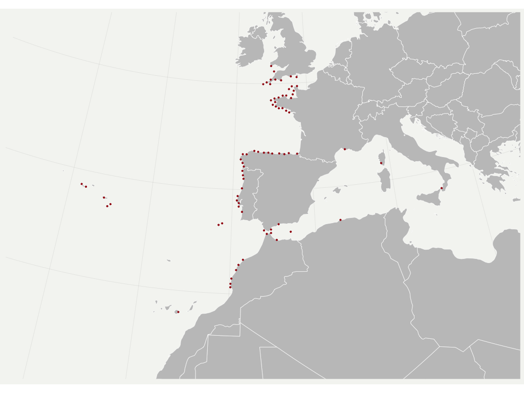
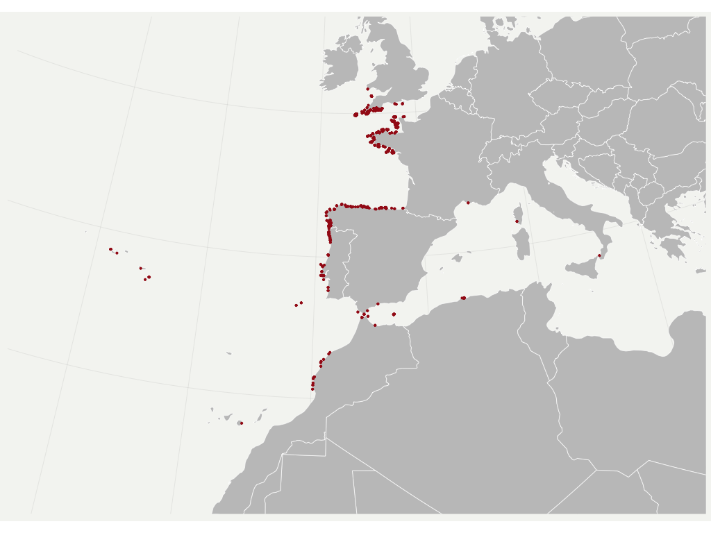
We propose a straightforward approach to reduce the effect of SA in SDM (see also Boavida et al., 2016 for more details). I use a simple example bellow focused on a brown algae species capable of producing marine forests and a set of environmental predictors known to largely explain its distribution.

1. A correlogram is produced to assess the correlation of each variable predictor within a range of geographic distances.

2. For each distance class, a linear model tests the effect of correlation with geographic distance. This finds the minimum non-significant autocorrelated distance.

3. The average of the minimum non-significant distances found per variable is used to prune the occurrence records, by leaving only one record within such distance.